UPDATE 3/28/2018: See Extracting MORE Features from Map Services to get around the maximum record count limit.

ArcGIS Server map services are a pretty cool thing.  Someone else is providing GIS data for you to consume in a map or application.  And if they keep it up to date over time, even better.

However, there are some times when you just need the data instead so you can edit/manipulate it for your GIS analysis needs.  If you cannot acquire a shapefile or geodatabase, there is a way to extract the features from a map service.

For you to extract the features, there must be three things in place:

• You must have access to the REST interface for the map service
• The layer in the map service that you want must be a feature layer
• The layer must have a query option with JSON format supported

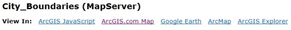
To demonstrate this, let’s head on over to the map services provided by Southern California Association of Governments (SCAG).  Specifically, the one for city boundaries:

http://maps.scag.ca.gov/scaggis/rest/services/City_Boundaries/MapServer

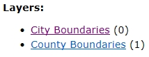
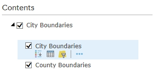
Since we have access to the REST interface, we can check out the different settings of the map service.  Note there are two layers, City Boundaries (layer 0) and County Boundaries (layer 1).

We are interested in the City Boundaries layer, so click on it.  This brings up detailed information about the data.

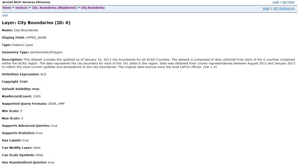
They were good to include when the data was updated in the Description.  Also note that it is a feature layer and we can query it.  If you scroll down to the bottom you will see the query option in the Supported Operations section.

Also listed at the bottom are the fields associated with the features.  We should take a look at these next to see what fields we want.  To do this, go back to the previous page and then click on the ArcGIS.com Map option in the View In section at the top:

This will open up a default map on ArcGIS Online and display the map service layers.

Click on City Boundaries to view the two layers, then click on the icon that looks like a spreadsheet just below the City Boundaries layer.

This will bring up the attribute table for the city boundaries.

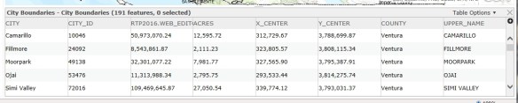
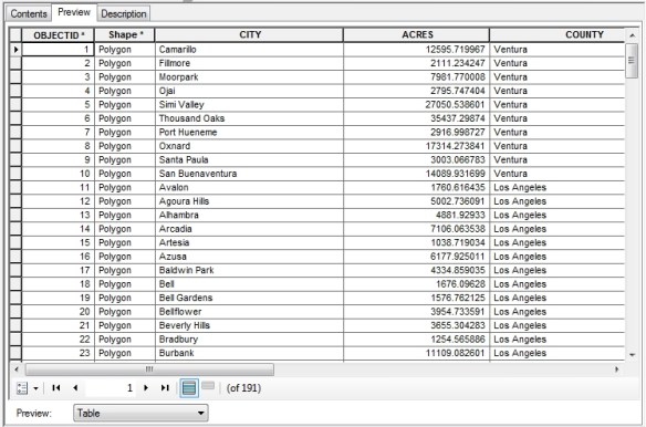
After taking a look at the data, all I want are the CITY, ACRES, and COUNTY fields.

Now let’s go back to the REST interface for the City Boundaries layer.  Take a look at the MaxRecordCount setting.  It is set to 1000.  This means that only 1000 records (features) can be returned for each query.  This can be extra work for you if this map service has more than 1000 features.  We need to find out how many features there are.  To do this, scroll to the bottom and click on the Query link in the Supported Operations section.  This will bring up the query interface for the map service.  This allows you to do a lot with the map service and get different results.  I will not go into the details of each parameter.  You can find out more info about them from the ArcGIS REST API reference.  For now, just enter “1=1” (without the quotes) in the Where input field.

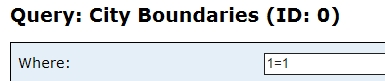
This is a little trick to return as many records as we can.  Also make sure to set Return Geometry to False and Return Count only to True.  With Return Count only set to True, we will actually get all records (an exeption to the MaxRecordCount setting).  Once those are set, click the Query (GET) button at the bottom of the query form.  It looks like nothing happened, but scroll down to the bottom to see the result.

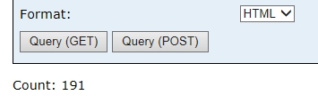
Note the count is 191.  So we don’t have to be concerned with the 1000 record limit.  We will be able to grab all the features at once.

NOTE: For those of you that are curious about the query, take a look at the URL in your web browser.  This is the REST query syntax used to get the record count.  We will be using something similar in a Python script to extract the actual geometry of all features.  You can mess around with the query form to see what happens and the URL that is created to make that happen.

We will be using a Python script to extract the features from the map service and create a featureset in a geodatabase.  Here is the script:

import arcpy

arcpy.env.overwriteOutput = True

baseURL = "http://maps.scag.ca.gov/scaggis/rest/services/City_Boundaries/MapServer/0/query"
where = "1=1"
fields = "CITY,ACRES,COUNTY"

query = "?where={}&outFields={}&returnGeometry=true&f=json".format(where, fields)

fsURL = baseURL + query

fs = arcpy.FeatureSet()
fs.load(fsURL)

arcpy.CopyFeatures_management(fs, "H:/scag/data.gdb/city_boundaries")

So what does this do?  First it loads the arcpy module and sets the overwrite option to True in case we want to run it again and overwrite the featureset.  A baseURL variable is set to the query URL of the city boundaries map service, a where variable for our where clause for the query, and a fields variable with a comma delimited list of the fields that we want.

Next a query variable is set with the actual query needed to extract the features.  Note the query is in quotes with {} for values that are plugged in by the variables listed in format() at the end.  Also note the returnGeometry parameter is set to true and f (for response format) is set to json.  What this query will do is extract all the records with just the fields we want, return all the geometry (the polygons), and output the whole thing in JSON format.  With the baseURL and query variables set, we merge them together for one long query URL as the fsURL variable.

Finally, we create an empty featureset (the fs variable), load the returned JSON data from the map service query into it, then copy it as a featureset to our geodatabase.

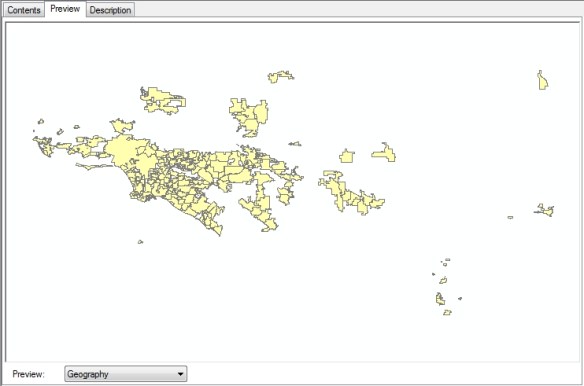
It takes a second or two to run the script.  Check out the result!

And here are the attributes we wanted for all 191 records.

I do want to point out that the data you get will be in the same projection as the map service.  You can find out what projection the map service is in by looking at the Spatial Reference setting in the REST interface.  Note this map service is using 26911:

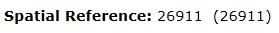
What the heck is that?  Go over to spatialreference.org and enter the number in the search field.  It will tell you this is the NAD83 UTM zone 11N projection.  If you wanted something else, like NAD83 California State Plane zone 5 US feet (2229), you would edit the Python script to include the output spatial reference parameter in your query, like this: “&outSR=2229”.  The data is projected on the fly for you and saved to your geodatabase!

I hope this helps you out when you are looking for data in map services.  -mike