I will start off the bat here and say I despise the Web Mercator projection. Web Mercator is a mathematically flawed version of the world Mercator, though it is used primarily in web based mapping programs.

Web Mercator really does not have a place here for me in local government. Because I deal with a more local scale (I use the California State Plane Coordinate System), the more global scale Web Mercator does not make sense for me to use. However, the likes of Google, Bing Maps, and ESRI following Google’s lead, kind of forces you to accept the projection if you want to use their services in your applications.

And then there is the history behind the confusing EPSG code used for the Web Mercator projection. Back in 2005, developers started projecting their own spatial data to overlay on Google and Bing Maps. EPSG was rather dismissive of the system used by Microsoft and Google and refused to assign it an official EPSG code. Their statement:

“We have reviewed the coordinate reference system used by Microsoft, Google, etc. and believe that it is technically flawed. We will not devalue the EPSG dataset by including such inappropriate geodesy and cartography.”

As a result developers needed some other way to refer to the projection used by Google Map, so Google came up with the code 900913 (i.e. GOOGLE) and it was commonly used. Aren’t they smart? This code was never developed or supported by the EPSG. However, in 2008 EPSG finally gave in and assigned it the code 3785, though they added the note “It is not a recognized geodetic system”.

But then just one year later, EPSG deprecated the 3785 code and issued a new code of 3857. The new code number was such a close permutation of the previous code that if you quickly glanced at the two numbers, they might look similar. Adding to the confusion many sites on the internet incorrectly listed the parameters of one code with the other code.

But I digress … so here is a good example why I don’t like Web Mercator and how I worked around it.

Los Angeles County built a map service of the preliminary 2014 aerial photography and allowed LARIAC members access to it. I am very thankful that they did this since I really needed early access to the new aerial photography. However, they created their map service using the Web Mercator projection.

If you use ArcMap to display the map service, you can set whatever projection you want and it will reproject the map service for you. That is great for our ArcMap users, but not so great for our internal applications. The applications require all data layers to be in the same projection. Since I use California State Plane Coordinates (specifically EPSG 2229), the county map service will not display in the application. What to do, what to do?

It was time for a hack! I’m basically going to create my own map service of the aerial photography in the projection I need.

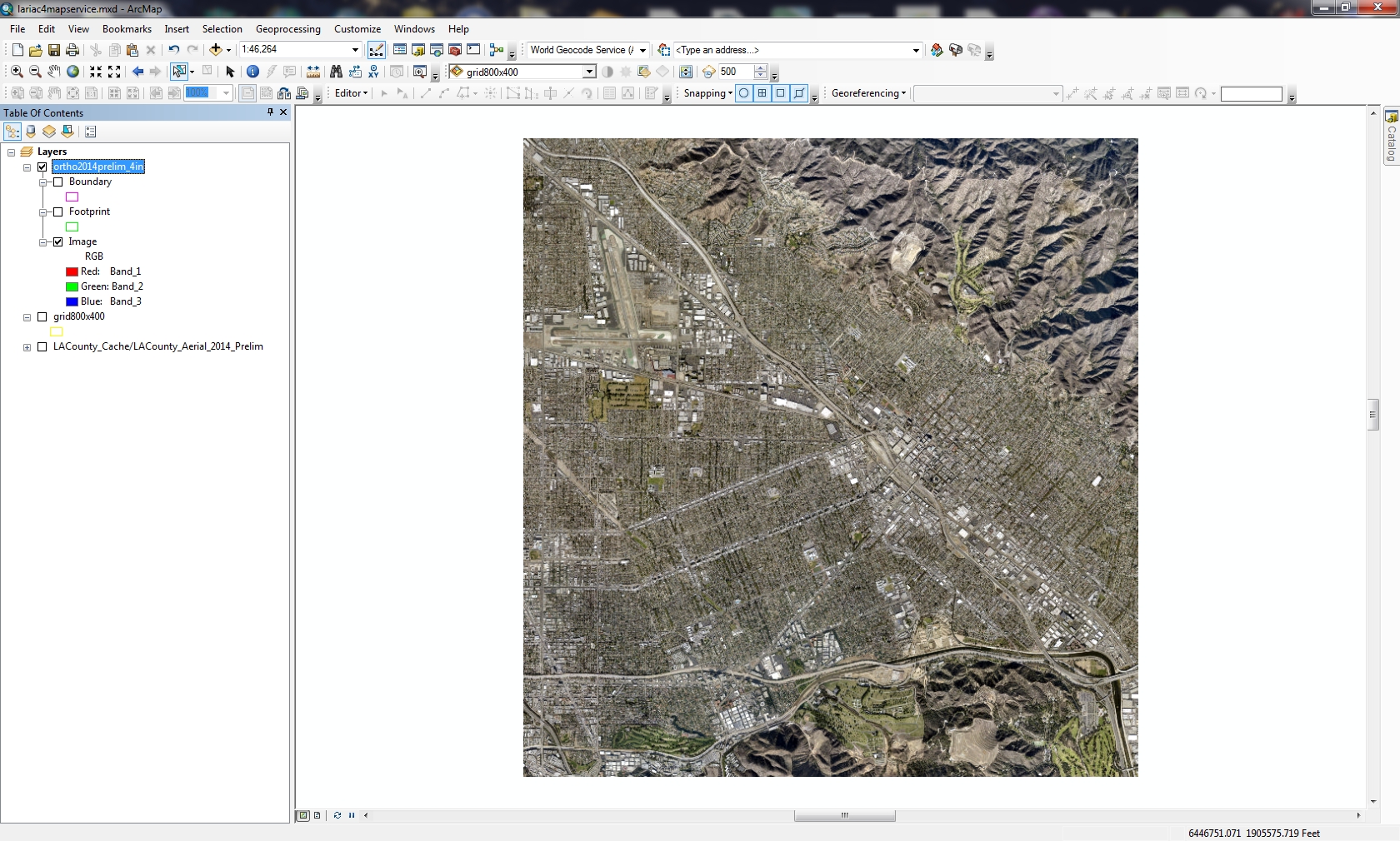
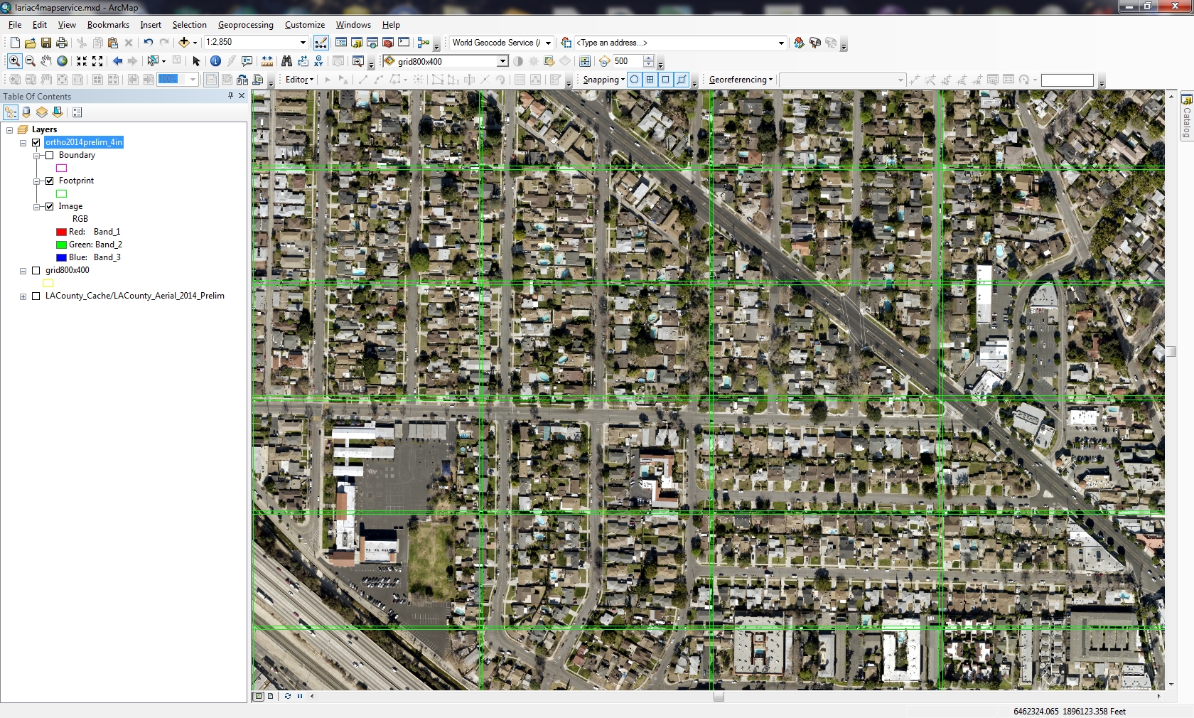
First I opened up ArcMap and brought in our city boundary layer. This set the projection to what I use. I then added the county map service and it was reprojected to match.

Note the Layer properties are set to the projection I want.

Next I buffered the city boundary by 1000ft. I will want my aerials to go a little beyond my border.

Now for the index grid. I first looked at the properties of the county map service to note the scale for the most detailed resolution, in this case 1:564. Also I noted the DPI used, in this case 96.

Next I maximized my ArcMap window and closed the TOC and other extraneous menus to get a full view, then zoomed to the scale 1:564.

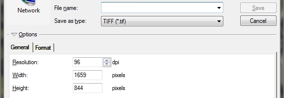
Next I selected File > Export Map and set it to TIFF and changed the Resolution setting to 96 DPI. This gave me the size of the image in pixels that I am currently viewing in ArcMap, in my case 1659 x 844.

Note that if you have a larger or higher resolution monitor, your pixel size will probably be a lot larger than mine.

Next I used the measurement tool to get the dimensions of the display window in map units. Mine came out to be about 810 feet wide by 412 feet tall.

I then rounded down the dimensions I will use to 800 feet wide and 400 feet tall. This will make the index grid polygons a little smaller than the display to allow for a little overlap when exporting.  This will become clearer in a moment.

I then used the Grid Index Features tool to create a grid that will be used to create each image tile.

I used the 1000ft buffer polygon as the input features, set the polygon width to 800 feet and height to 400 feet, and unchecked “Generate Polygon Grid that intersects input feature layers or datasets” (I wanted grid cells that fell outside my buffered area). What resulted was a nice grid that will be used to generate the image tiles.

Note that when I zoom to a tile and set the scale to 1:564, you can see the overlap that will be used for each image. It is important to have this overlap when exporting the images.

I then opened my TOC to remove all layers except the polygon grid and the map service. I also made sure to “uncheck” the polygon grid layer so it would not draw. I then removed the TOC again to get the maximum display in ArcMap as before.

Now for the fun stuff.

I used the Python scripting window in ArcMap to automate the process of zooming to each tile at a scale of 1:564, then exporting the display to a GeoTIFF file using the name stored in the tile grid polygon. Here is my python code that did it:

mxd = arcpy.mapping.MapDocument("CURRENT")
df = arcpy.mapping.ListDataFrames(mxd)[0]
df.scale = 564
gridlayer = arcpy.mapping.ListLayers(mxd, "grid800x400", df)[0]
arcpy.SelectLayerByAttribute_management(gridlayer, "NEW_SELECTION")
for row in arcpy.SearchCursor(gridlayer):
  df.panToExtent(row.shape.extent)
  arcpy.RefreshActiveView()
  filename = "H:/airphoto/2014/images/" + \
    str(row.getValue("PageNumber")).zfill(4) + ".tif"
  arcpy.mapping.ExportToTIFF(mxd, filename, df, df_export_width=1659, \
    df_export_height=844, geoTIFF_tags=True)

Note my polygon grid layer was named “grid800x400”.

So what does this do? It first sets the mxd variable to the current ArcMap session, then sets the data frame variable df to the first layer name (which when you open ArcMap the default name is Layer), and then the data frame’s scale is set to 1:564.

Next the gridlayer variable is set to the polygon grid layer, which is the first layer in the data frame TOC. The script then selects all the grid polygons and then using cursors, steps through each record (polygon) to pan to it (thus keeping the scale set to 1:564), refreshes the display for the new view, and then using the value in the PageNumber field exports a uniquely named GeoTIFF file using my specified dimensions. Note that zfill(4) will pad a string to the left with zeros to fill the width of 4, so the PageNumber value of 5 will become 0005 and the GeoTIFF file name will be named 0005.tif.  Fancy!

If you modify this code for your environment, then copy and paste it in the Python window, you can sit back and watch this run, zooming to each tile and exporting the display to a GeoTIFF file. It took about an hour to create 2849 images, 11.9 GB total.

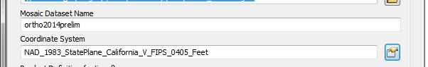
Now what? You have to put all the images together to make a seamless image. To do that I created a Mosaic Dataset. Using ArcCatalog I created a new file based geodatabase. Then in it created a new Mosaic Dataset. The Create Mosaic Dataset tool will ask for a name and coordinate system.

Once created, I then added my tiff images to the Mosaic Dataset. Also make sure to define and build overviews (images for other scales). In the end you get something that looks like this:

Turn on the footprints to see the individual image tiles that make up the mosaic.

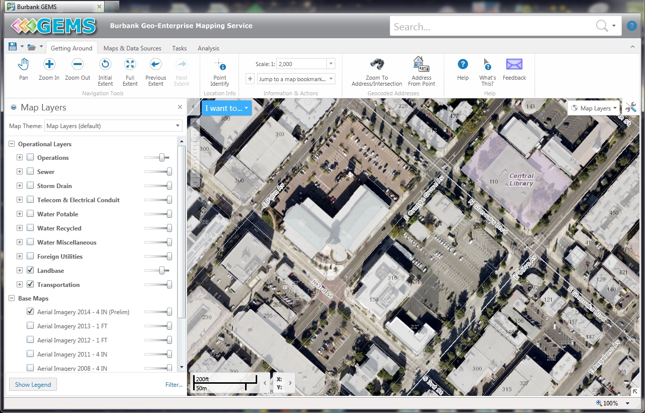
Now all there is left to do is create an MXD of just the mosaic dataset and publishing a map service of the new image. I will not go into the details of doing that. In the end I now have a map service in the proper projection that will work for my internal applications. Looky here:

Take that Web Mercator!  -mike