Changing a Field’s Length

From time to time I encounter the issue of a text field that is too small.  A great example would be a street name field that was fine for a while, but now you have new street names that require more characters.  Here are a few examples on how to change the field length.  I will be using ArcGIS 10.2.2 and a feature class in a file geodatabase to demonstrate.

The Traditional Way

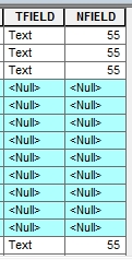
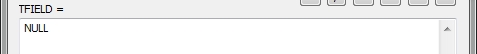
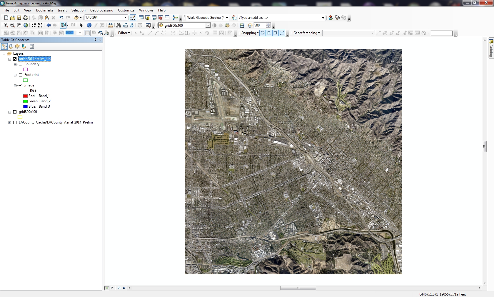
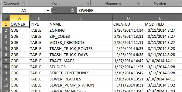
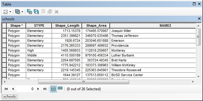
Open the feature class in ArcMap and bring up the attribute table.  Below is a feature class representing schools.

fieldlen1

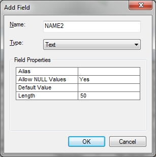
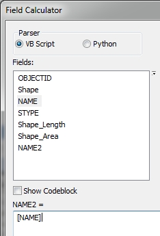
Add a new text field to the table with more characters.

fieldlen2

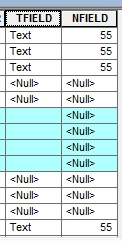
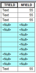
Right click on the new field name in the table and select the field calculator option to calc the new field to the old one.

fieldlen3

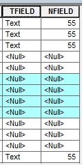
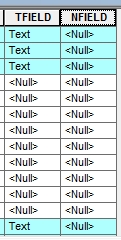
And finally right click on the old field name and delete it.  Here is mine.

fieldlen4

What I don’t like about this method is that I could not reuse the field “NAME” and had to create “NAME2”.  Also I liked the original order, and now my field is at the end of the table.  Sure, I could do it again by adding back the field name “NAME” and recalcing again, but my field is still at the end.  Yes you can reorder fields for display in ArcMap, but it does not do anything to the real order of the fields in the geodatabase … and that bugs me!  So on to the second option.

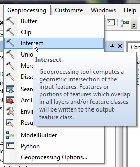
The Feature Class to Feature Class Tool

A better way of doing this is by using the Feature Class to Feature Class tool.  The tool allows you to change the field mapping, thus allowing you to change the field length and keep the field name and position if you want.  You can find the tool by doing a tool search.  Open the tool and load in your input feature class.

fieldlen5

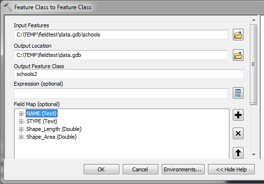
You have to specify a new output feature class.  Also note the fields that are listed in the field map section.  Right click on the field you want to change the length of and select Properties.

fieldlen6

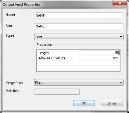
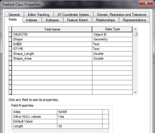
Change the Length property and click OK.  Then click OK on the tool.  A new feature class is created with the larger field.  Just to verify, you can use ArcCatalog to view the field information.

fieldlen7

Field mapping with the tool allows you to shuffle around the fields, rename them, or remove ones you do not want as well.  The down side?  A new feature class has to be created, which might be an issue if you have millions of records and limited space, however you probably don’t so it works out fine.

After the tool is done, you can delete your old feature class and rename the new one to whatever you want.

So now that leaves the last option … a python script that will do this.

The Python Script

# Change a text field length

# Import arcpy module
import arcpy

# Overwrite exising output
arcpy.env.overwriteOutput = True

# Setup feature class and field info
infc = "c:/temp/fieldtest/data.gdb/schools"
outloc = "c:/temp/fieldtest/data.gdb"
outfc = "schools2"
fieldname = "NAME"
fieldlen = 50

# Setup field mappings
skipfields = ["OBJECTID", "FID", "Shape"]
fms = arcpy.FieldMappings()
fields = arcpy.ListFields(infc)
for field in fields:
  if field.name in skipfields:
    pass
  else:
    fm = arcpy.FieldMap()
    fm.addInputField(infc, field.name)
    if field.name == fieldname:
      newfield = fm.outputField
      newfield.length = fieldlen
      fm.outputField = newfield
    fms.addFieldMap(fm)

# Copy feature class with new field mappings
arcpy.FeatureClassToFeatureClass_conversion(infc, outloc, outfc, field_mapping=fms)

# All done!
print "Done!"

So let’s step through this.  The arcpy module is imported and we set our overwrite output to True so we can rerun this script and overwrite our output feature class.

Next are some variables that you can modify.  The input feature class “infc”, the output location “outloc”, the output feature class name “outfc”, the text field “fieldname” that we want to change the length of, and the new field length “fieldlen”.

Next, we setup field mappings, but we only want the non-system type fields.  Fields like OBJECTID, FID, and Shape are maintained by ArcGIS, so we don’t want to mess with them.  A list of fields we want to avoid, “skipfields”, is set, a blank field mappings “fms” is set, and we collect all the fields in the input feature class and store them in “fields”.

Next, we loop through all the fields and check if each one is a field we should skip.  If so, we do nothing “pass”.  If not, we setup a blank field map “fm”, add all the field information to it (field type, length, etc.) from the field in the input feature class, then check if the field is the one we need to change.  If so, we make a new field variable “newfield” set to the current field map, change the length property of the “newfield” to the value we set in “fieldlen”, then reset the current field map to our “newfield” setting.  We then add the field map to the field mappings “fms”.  Think of the field mappings as the list of fields and their properties, while a field map is the properties of one field.

Once the loop is done building the field mappings “fms”, it is used in arcpy.FeatureClassToFeatureClass_conversion to create our new feature class “outfc”.

Give the script a try and see if it works for you.  One thing you could do with the script at the end is to rename or delete the old input feature class and then rename the new output feature class to the old name.  Just a thought!  -mike

Displaying CIR from 4-band NAIP

For those of you viewing the 4-band NAIP image services in ArcGIS Desktop, you can put the 4th band to work and view the imagery as Color Infrared (CIR).

First to get the 4-band NAIP image service into ArcGIS Desktop (I’m using 10.2.2), click on the Add Data button and select “GIS Servers” from the “Look in” pulldown menu.  Then double click on “Add ArcGIS Server” in the list.

naip1

You will be asked what you would like to do, so select “Use GIS services” and click the Next button.  Then in the Server URL input field, enter the following:

naip2

Click the Finish button and the image service will be added to your list of GIS Servers.

naip3

Double click on it to reveal the folders.  Double click on the NAIP folder to list the different image services.  Double click on one to add as a layer in ArcMap.

naip4

What you are currently viewing is Natural Color or RGB.  You are viewing 3 of the 4 bands, or the Red, Green, and Blue bands.  Here is a nice graphic of the visible spectrum:

Together the 3 bands make the natural color image.  Right click on the NAIP layer in ArcMap and select Properties.  Click on the Symbology tab to view the bands being used.

naip6

Note the image service was initially setup with a Minimum-Maximum stretch.  Depending on the imagery, you can fiddle with the stretch to make the colors more pleasing.  The setting here seems to make the imagery a little more brighter, though I like it better with it set to “None”.

naip7

Now for the fun.  You need to shift around the bands to view the imagery in CIR.  To do that, there is a pulldown for each of the bands.  Make the Red channel Band 4, the Green channel Band 1, and the Blue channel Band 2.  Band 3 is not used.

naip9

Click OK or Apply to view the Color Infrared.

naip8

Nice!

I think the best part of this is that for LARIAC participants in LA County, we can take advantage of this free source since we did not get CIR imagery this time around.  Though this is only 1 meter resolution, it might help out some people that need this information.  And besides, it matches the year our latest 4in resolution imagery was taken.

I bet there is a way to “enhance” the CIR imagery with LARIAC’s imagery … that is using high-resolution panchromatic imagery to sharpen multi-spectral imagery.  If someone wants to do that, please do a writeup using LARIAC imagery and NAIP!  -mike

ArcMap: Dealing with NULLs

NULL values in GIS data can trip you up if you don’t know how to deal with them.  A NULL value is not the same as a blank (empty) value, and actually takes up 1 bit more of space than an empty value.  Allowing a field to be NULL introduces an additional state that you would not have if the field was created to not allow NULLs.  And yes, you can have NULLs in numeric fields too!

Why have a NULL value in your data?  Usually this is used to mean “not set” or “uninitialized”.  A good example would be an employee database with a termination date field that is set to NULL when the employee is new.  Another example would be an elevation field.  You could use a NULL value to represent “not known”, since zero is a valid elevation.  More than likely you have fields that allow NULLs because someone created them not paying attention to the defaults.

So how do you specify a field to allow NULLs or not?  Open ArcMap (I’m using version 10.2.2) and bring in some data from a geodatabase.  Then open the data’s attribute table and select “Add Field…” from the Table Options icon.

nulls1

Note by default in the Field Properties that “Allow NULL Values” is set to “Yes”.  If you do not want NULLs, set it to “No”.  If you set it to “No” and do not specify a “Default Value”, then Text fields will default to a blank (empty) value and numeric fields will default to zero.  Also, keep in mind that you can add a field with “Allow NULL Values” set to “No” only if your feature class or table is not populated yet with records.

So let’s take a look at some test data I created with some fields that allow NULLs.

nulls2

As you can probably guess, the field TFIELD is a text field and NFIELD is a numeric field.  Note some records have NULL values while others have data.

Using the Select By Attributes tool, I can select NULL values in the TFIELD by constructing the following SQL expression.

nulls3

The records with NULL in the TFIELD are selected.

nulls4

If I wanted to select everything but NULL, I would have used this SQL expression.

nulls5

nulls6

Numeric fields work the same way when selecting NULLs.

nulls7

nulls8

Now let’s take a few records and calc the TFIELD value to blank.  First I select a few records.

nulls9

Then right click on the TFIELD name in the attribute table and select “Field Calculator…”.  Then in Field Calculator I specify TFIELD = “” (that is two double quotes with no space between them).

nulls10

Note the values change from NULL to blank.

nulls11

Now let’s select NULL values in TFIELD again with the Select By Attributes tool using “TFIELD IS NULL”.  Look what happens.

nulls12

Note the blank records were not selected.  This shows that blanks are not the same as NULLs.  You have to be careful of this.  If you wanted all blanks and NULLs, try this expression in the Select By Attributes tool.

nulls13

Note in this tool I had to use two single quotes with no spaces between for the SQL expression.  This selects all NULLs and blanks.

nulls14

What if I wanted to calc a NULL value to a field?  First I will select some records, like my blank values in the TFIELD, then using the Field Calculator I specify TFIELD = NULL.

nulls15

nulls16

I can do the same for the numeric field.  First I will select all records with the value of 55.

nulls17

Then using the Field Calculator I specify NFIELD = NULL.  All values of 55 are changed to NULL.

nulls18

So there you have it.  You are now an expert with dealing with NULLs and hopefully when you setup your data, you will know when to use them and NOT NULL!

Hacking Web Mercator Map Services

I will start off the bat here and say I despise the Web Mercator projection. Web Mercator is a mathematically flawed version of the world Mercator, though it is used primarily in web based mapping programs.

Web Mercator really does not have a place here for me in local government. Because I deal with a more local scale (I use the California State Plane Coordinate System), the more global scale Web Mercator does not make sense for me to use. However, the likes of Google, Bing Maps, and ESRI following Google’s lead, kind of forces you to accept the projection if you want to use their services in your applications.

And then there is the history behind the confusing EPSG code used for the Web Mercator projection. Back in 2005, developers started projecting their own spatial data to overlay on Google and Bing Maps. EPSG was rather dismissive of the system used by Microsoft and Google and refused to assign it an official EPSG code. Their statement:

“We have reviewed the coordinate reference system used by Microsoft, Google, etc. and believe that it is technically flawed. We will not devalue the EPSG dataset by including such inappropriate geodesy and cartography.”

As a result developers needed some other way to refer to the projection used by Google Map, so Google came up with the code 900913 (i.e. GOOGLE) and it was commonly used. Aren’t they smart? This code was never developed or supported by the EPSG. However, in 2008 EPSG finally gave in and assigned it the code 3785, though they added the note “It is not a recognized geodetic system”.

But then just one year later, EPSG deprecated the 3785 code and issued a new code of 3857. The new code number was such a close permutation of the previous code that if you quickly glanced at the two numbers, they might look similar. Adding to the confusion many sites on the internet incorrectly listed the parameters of one code with the other code.

But I digress … so here is a good example why I don’t like Web Mercator and how I worked around it.

Los Angeles County built a map service of the preliminary 2014 aerial photography and allowed LARIAC members access to it. I am very thankful that they did this since I really needed early access to the new aerial photography. However, they created their map service using the Web Mercator projection.

If you use ArcMap to display the map service, you can set whatever projection you want and it will reproject the map service for you. That is great for our ArcMap users, but not so great for our internal applications. The applications require all data layers to be in the same projection. Since I use California State Plane Coordinates (specifically EPSG 2229), the county map service will not display in the application. What to do, what to do?

It was time for a hack! I’m basically going to create my own map service of the aerial photography in the projection I need.

First I opened up ArcMap and brought in our city boundary layer. This set the projection to what I use. I then added the county map service and it was reprojected to match.

webmerc1

Note the Layer properties are set to the projection I want.

Next I buffered the city boundary by 1000ft. I will want my aerials to go a little beyond my border.

webmerc2

Now for the index grid. I first looked at the properties of the county map service to note the scale for the most detailed resolution, in this case 1:564. Also I noted the DPI used, in this case 96.

webmerc3

Next I maximized my ArcMap window and closed the TOC and other extraneous menus to get a full view, then zoomed to the scale 1:564.

webmerc4

Next I selected File > Export Map and set it to TIFF and changed the Resolution setting to 96 DPI. This gave me the size of the image in pixels that I am currently viewing in ArcMap, in my case 1659 x 844.

webmerc5

Note that if you have a larger or higher resolution monitor, your pixel size will probably be a lot larger than mine.

Next I used the measurement tool to get the dimensions of the display window in map units. Mine came out to be about 810 feet wide by 412 feet tall.

webmerc6

I then rounded down the dimensions I will use to 800 feet wide and 400 feet tall. This will make the index grid polygons a little smaller than the display to allow for a little overlap when exporting.  This will become clearer in a moment.

I then used the Grid Index Features tool to create a grid that will be used to create each image tile.

webmerc7

I used the 1000ft buffer polygon as the input features, set the polygon width to 800 feet and height to 400 feet, and unchecked “Generate Polygon Grid that intersects input feature layers or datasets” (I wanted grid cells that fell outside my buffered area). What resulted was a nice grid that will be used to generate the image tiles.

webmerc8

Note that when I zoom to a tile and set the scale to 1:564, you can see the overlap that will be used for each image. It is important to have this overlap when exporting the images.

webmerc9

I then opened my TOC to remove all layers except the polygon grid and the map service. I also made sure to “uncheck” the polygon grid layer so it would not draw. I then removed the TOC again to get the maximum display in ArcMap as before.

Now for the fun stuff.

I used the Python scripting window in ArcMap to automate the process of zooming to each tile at a scale of 1:564, then exporting the display to a GeoTIFF file using the name stored in the tile grid polygon. Here is my python code that did it:

mxd = arcpy.mapping.MapDocument("CURRENT")
df = arcpy.mapping.ListDataFrames(mxd)[0]
df.scale = 564
gridlayer = arcpy.mapping.ListLayers(mxd, "grid800x400", df)[0]
arcpy.SelectLayerByAttribute_management(gridlayer, "NEW_SELECTION")
for row in arcpy.SearchCursor(gridlayer):
  df.panToExtent(row.shape.extent)
  arcpy.RefreshActiveView()
  filename = "H:/airphoto/2014/images/" + \
    str(row.getValue("PageNumber")).zfill(4) + ".tif"
  arcpy.mapping.ExportToTIFF(mxd, filename, df, df_export_width=1659, \
    df_export_height=844, geoTIFF_tags=True)

Note my polygon grid layer was named “grid800x400”.

So what does this do? It first sets the mxd variable to the current ArcMap session, then sets the data frame variable df to the first layer name (which when you open ArcMap the default name is Layer), and then the data frame’s scale is set to 1:564.

Next the gridlayer variable is set to the polygon grid layer, which is the first layer in the data frame TOC. The script then selects all the grid polygons and then using cursors, steps through each record (polygon) to pan to it (thus keeping the scale set to 1:564), refreshes the display for the new view, and then using the value in the PageNumber field exports a uniquely named GeoTIFF file using my specified dimensions. Note that zfill(4) will pad a string to the left with zeros to fill the width of 4, so the PageNumber value of 5 will become 0005 and the GeoTIFF file name will be named 0005.tif.  Fancy!

If you modify this code for your environment, then copy and paste it in the Python window, you can sit back and watch this run, zooming to each tile and exporting the display to a GeoTIFF file. It took about an hour to create 2849 images, 11.9 GB total.

Now what? You have to put all the images together to make a seamless image. To do that I created a Mosaic Dataset. Using ArcCatalog I created a new file based geodatabase. Then in it created a new Mosaic Dataset. The Create Mosaic Dataset tool will ask for a name and coordinate system.

webmerc10

Once created, I then added my tiff images to the Mosaic Dataset. Also make sure to define and build overviews (images for other scales). In the end you get something that looks like this:

webmerc11

Turn on the footprints to see the individual image tiles that make up the mosaic.

webmerc12

Now all there is left to do is create an MXD of just the mosaic dataset and publishing a map service of the new image. I will not go into the details of doing that. In the end I now have a map service in the proper projection that will work for my internal applications. Looky here:

webmerc13

Take that Web Mercator!  -mike

Changing Data Paths in MXD Files

So you moved your GIS data and now you need to update your MXD files with all those layers that point to the old data location.  What to do?  Use ArcCatalog to update them.  I’m using version 10.2 here.

First open ArcCatalog and navigate to the location of your MXD files.  Next, right click on one of the files and select “Set Data Source(s)…”

mxd1

You can then edit your data paths by selecting the ones that need editing, then pressing the Replace button:

mxd2

After you change the paths, make sure to enter a new MXD file name, then press the OK button.  That’s it!

Trying Out 64-bit Background Geoprocessing for ArcGIS Desktop

ArcGIS Desktop is a 32-bit application. Background processing was introduced at the 10.0 release which allowed you to run geoprocessing tasks as a background process. This freed you up to do other things while your process was working away in the background. However, this background process still ran in the 32-bit world.

At version 10.1 SP1, 64-bit background geoprocessing was introduced. If you had a 64-bit PC, you could install this extra piece of software to take advantage of your 64-bit architecture.

Installing 64-bit background geoprocessing will replace your current 32-bit background geoprocessing. All scripts, models, and tools which execute in the background will use a 64-bit process. Your biggest benefit when using 64-bit background processing is that your large 64-bit processes can take advantage of more memory (if available) than when using 32-bit processes (the 3gb barrier).

So let’s get started. First, you will need a 64-bit PC that has ArcGIS Desktop 10.1 or higher installed on it. You will also need a process that takes some time to run, so you can compare before and after installing the 64-bit background geoprocessing software.

I chose to use ArcCatalog 10.2 in my test. Make sure to enable Background Geoprocessing in the Geoprocessing Options menu (accessed under Geoprocessing > Geoprocessing Options).

64bit-settings

For my test, I chose to use the Intersect Tool under the Geoprocessing pulldown menu in ArcCatalog.

64bit-intersect

I will be intersecting a 5 mile buffer of street centerlines from the City of Burbank with 10 foot contour lines from all of LA County. There are 28,817 records (6.10mb) for the street centerline data, and 1,131,734 records (2.34gb) for the contour lines.

64bit-arcmap

Why would I want to do this? I don’t know, but I wanted two large data sets to try this on.

After adding the two data sets to the Intersect Tool, I ran the tool and it took off running in the background.  Bringing up the Windows Task Manager shows my CPU and memory usage during the run.

64bit-process1

I could see the process seemed to only take up 3 of the 4 CPU cores and memory usage was constant.  I had other programs open at the time so memory usage was up more than usual.  Once the tool finished, the results could be displayed in the Geoprocessing Results window (accessed under Geoprocessing > Results).

64bit-results1

The intersect process took 7 minutes and 30 seconds to complete using 32-bit background geoprocessing.

Ok, so now let’s install the 64-bit Background Geoprocessing software. Close all ArcGIS applications first. Find your ArcGIS Desktop CD or you can download just the 64-bit Background Geoprocessing install file from ESRI’s customer care site.  I have the CD, so I start it up and choose 64-bit Background Geoprocessing.

64bit-install

During the install, two things happen. The 64-bit binaries for Desktop are installed under your_arcgis_software_location/ArcGIS/Desktop10.2/bin64 and 64-bit Python is installed under your_python_directory/ArcGISx6410.2. I will talk about Python later and things you should be aware of after this install.

Now with 64-bit background geoprocessing installed, I startup ArcCatalog and run the Intersect Tool again to see if processing is faster.  While it ran, I did notice all 4 CPU cores were utilized, CPU usage went up, and more memory use and fluctuation.

64bit-process2

And here are my results:

64bit-results2

My process ran a little faster lasting 6 minutes and 14 seconds, or 1 minute and 16 seconds faster. An almost 17% improvement.  Frankly I was expecting something like half the processing time. Maybe a better test would be using a 32-bit PC and compare to a 64-bit PC. I just had my 64-bit PC to compare both, so maybe it was helping the 32-bit process a little.  Not sure.  Please post a comment if you have an idea why.  I have heard that with 64-bit processing you can see a 20% improvement.

Now for Python. As stated earlier, the 64-bit version of Python gets installed as well. This is for the geoprocessing tools in ArcGIS Desktop. If you are into writing Python scripts, and you want to take advantage of 64-bit, you will need to make sure to run your scripts against 64-bit Python.

Typically the last version of Python installed, by default, will be the one you execute against when double clicking a python script from Windows Explorer. If you last installed 64-bit Background Geoprocessing, you will probably be executing against 64-bit Python. You can always change which program executes when double clicking a file in Windows.

When I open my Python window, I see that it is running the 64-bit version.

64bit-python64

Keep in mind that if you installed 3rd party Python tools, you will need to get the 64-bit versions. For example, if you installed SciPy, you will need to download and install the 64-bit version as well.

Also, if your background processes (or stand alone Python scripts) accesses data in an Enterprise Geodatabase, like SQL Server or Oracle, you will need to install the 64-bit client libraries for those databases on your PC so the process/script can connect to those databases.  ArcGIS Desktop will continue to use the 32-bit libraries, and background processes/stand alone Python scripts will use the 64-bit libraries.

Lastly, if you uninstall the 64-bit Background Geoprocessing program, I found that when I tried to double click a Python script, it could not find the 32-bit Python program.  I had to re-associate .py files to the 32-bit executable.  ArcGIS Desktop seemed to work fine though.

If you have not taken advantage of 64-bit Background Geoprocessing for ArcGIS Desktop, you really should. Even though my simple test showed it helped a little, anything I can do to make my processes run faster, even by a minute, will help in the long run. Give it a try and see if it helps you out. For more info, visit the 10.2 Help on Background Geoprocessing.  -mike

ArcMap: I Just Want the XY

How many times while working in ArcMap have you had the need to find the XY coordinate for a certain location? Sure you can hover over the map with your mouse and read the coordinates displayed in the lower right hand corner of the ArcMap window:

xy1

But depending on your projection, those coordinates might not be in the format you want. For example, you want longitude and latitude but your coordinates are displayed in another projection system.

Here comes the Identify tool to the rescue! Identify tool you ask? Yes, besides displaying what features you clicked on it also displays the coordinates where you clicked. You have been using this tool for a long time but maybe overlooked the coordinate display. Try it now. Here is what I got:

xy2

Note “Location:” just above the field and value listing. If you want to change the coordinate format, click on that little down arrow next to the coordinate display:

xy3

Now pick something else, like Decimal Degrees and see your new coordinates:

xy4

You can even copy what is displayed and paste it in something else, like an email or a report.

So there you go, a quick way of getting point and click XY coordinates from ArcMap. Enjoy! -mike

SDE Geodatabase Feature Class: Where is the Modified Date?

Have you ever tried using ArcCatalog to look at a listing of your feature classes in an SDE Geodatabase to see when they were modified, only to be disappointed that no dates are displayed?  I was:

sdefc1

If you’ve been around a while, remember that 1984 Wendy’s commercial with the old lady that kept saying “Where’s the beef?”:

Yeah ESRI, where’s the beef?  You do this for a File Geodatabase:

sdefc2

Why not for SDE?  Sure, I can use versioning and look for the date that way, but we are a small GIS shop here and only a few people do the editing anyway.  What to do?

After talking with our friendly Oracle DBA, searching through some system tables, searching the ArcPy classes, and working on a SQL query, I finally came up with a nice Python script that will pull out the SDE Geodatabase feature classes (they are just tables) and list the creation and modification dates.  The info is also saved to a CSV file so you can open it up in Excel.

Here is the script, free for you to use.  ** See update 12/4/2017 in comments section **

# ---------------------------------------------------------------------
# get_sde_date.py
# Created on: 3/26/2014
# By: Michael A. Carson, GIS Manager, City of Burbank GIS
# Description: Queries SDE GDB in Oracle to get feature class table dates.
# ---------------------------------------------------------------------

# Import modules
import arcpy,sys,csv

# Python environment
arcpy.env.overwriteOutput = True

# Local variables
sde_conn_file = r"H:\testdir\sde_gdb_connection.sde"
output_file = r"H:\testdir\sde_fc_tables.csv"
sql_statement = "select OWNER,OBJECT_TYPE,OBJECT_NAME,CREATED, \
    LAST_DDL_TIME from DBA_OBJECTS where OWNER = 'GDB' \
    and OBJECT_TYPE = 'TABLE'"

# Execute SQL statement and save table list
try:
    # Make data path relative
    arcpy.env.workspace = sys.path[0]

    # Use valid SDE connection file to connect to SDE GDB in Oracle
    sde_conn = arcpy.ArcSDESQLExecute(sde_conn_file)

    print("=============================================\n")

    print("Execute SQL Statement: {0}".format(sql_statement))
    try:
        # Pass the SQL statement to the database
        sde_return = sde_conn.execute(sql_statement)
    except Exception as err:
        print(err)
        sde_return = False

    # If the return value is a list, display each list as a row
    if isinstance(sde_return, list):
        for row in sde_return:
            print(row)
        f = open(output_file, 'wb')
        writer = csv.writer(f, delimiter=',')
        writer.writerow(['OWNER', 'TYPE', 'NAME', 'CREATED', 'MODIFIED'])
        writer.writerows(sde_return)
        f.close()
        print("Number of rows returned by query: {0} rows".format(len(sde_return)))
        print("=============================================\n")
    else:
        # If the return value was not a list, the statement was most likely a DDL statement
        if sde_return == True:
            print("SQL statement: {0} ran successfully.".format(sql_statement))
        else:
            print("SQL statement: {0} FAILED.".format(sql_statement))
        print("=============================================\n")

except Exception as err:
    print(err)

Keep in mind this is for an Oracle SDE Geodatabase.  I am also using ArcGIS 10.1.  It will probably NOT work for SQL Server or PostgreSQL.  Post a comment if you get it to work on those databases.

So how does this work?  Looking at the local variables section, you need to change the value for the sde_conn_file and sql_statement.  You can also change the output_file name if you want too.

# Local variables
sde_conn_file = r"H:\testdir\sde_gdb_connection.sde"
output_file = r"H:\testdir\sde_fc_tables.csv"
sql_statement = "select OWNER,OBJECT_TYPE,OBJECT_NAME,CREATED, \
    LAST_DDL_TIME from DBA_OBJECTS where OWNER = 'GDB' \
    and OBJECT_TYPE = 'TABLE'"

The script uses your SDE connection file to connect to the SDE Geodatabase … AS SDE.  This is important.  You must connect as the SDE user since the SDE user has privilages to read some of the Oracle system tables that store the info we want to extract.  So where can you find your connection file?  You probably used ArcCatalog to make your connection to the SDE Geodatabase.  Here are some of mine:

sdefc3

They are listed under Database Connections in the ArcCatalog Tree.  These connection files are located under your user directory (I’m assuming you are using Windows 7).  I found mine located under here:

C:\Users\mike\AppData\Roaming\ESRI\Desktop10.1\ArcCatalog\

The connection files are named the same as you see them in ArcCatalog.  I just copied the one that connects as the SDE user and copied it to my workspace for the script.  If you don’t want to copy the file, just set the sde_conn_file variable to point to wherever it is.  The nice part about using a connection file is that you don’t expose your SDE user password in the Python script.

Now the SQL statement:

sql_statement = "select OWNER,OBJECT_TYPE,OBJECT_NAME,CREATED, \
    LAST_DDL_TIME from DBA_OBJECTS where OWNER = 'GDB' \
    and OBJECT_TYPE = 'TABLE'"

Note the “\” is just a Python line continuation character that I used to make this fit in this blog (and still run in Python as you see it).  Normally I would have the whole thing on one line!  Anyway, here is where you want to modify the owner.  I have an owner, the database user named GDB, that I use to create and modify some of our feature classes in the SDE Geodatabase.  I want to pull out just those tables that are associated with user GDB.  If you have more users that edit data, you can change the owner part of the SQL statement this way:

(OWNER = 'USER1' or OWNER = 'USER2' or OWNER = 'USER3')

Everything else should stay the same.

Now run your Python script.  It should connect to your SDE Geodatabase using the ArcPy class ArcSDESQLExecute and your connection file, then execute the SQL statement, return a list of records with the owner name, object type, creation date, and date last modified, then write the list to the output CSV file.  Here is the output when I ran my script:

sdefc4

And here is my CSV file:

sdefc5

The one thing I don’t like is the default date/time format Excel sets for the CREATED and MODIFIED column.  To change it, I select both columns, right click to select Format Cells, then use a custom date/time setting like so:

sdefc6

You can pick from a list or enter what you want like I did.  Much better!

sdefc7

Remember, everything that is listed is a table.  Your feature classes are just tables as well.  You might notice in your output that there are tables listed that are not feature classes, like indexes (_IDX$) and location tables for geocoding (_LOX).  You could filter those out in your SQL statement.  For me, I like to see everything.

You could also modify this script and run it as a scheduled task for a monthly report, thus helping you identify a volume of modifications to your data over time.  Of course your friendly DBA could probably do that from the database side of things, but then you would not have fun doing this by yourself!

Please, if you modify the script to work with SQL Server or PostgreSQL, tell us how by posting a reply.  Did I mention that before?

So there you have it, the ability to get at the modification date for feature classes in an Oracle SDE Geodatabase.  Maybe ESRI will change it so we can see it in ArcCatalog in the next version?  Time will tell.  Enjoy.  -mike

My Adventure with Google Maps in ArcMap

Many years ago I wondered how to get Google Maps as a background map in ArcMap.  Why did I want to do this?  Because it would be cool and basemaps in ArcMap were limited back then.  However, I never had a chance to try it out … got too busy.  Besides, there are many options now for basemaps and better than Google Maps.  For a government agency, replacing authoritative GIS data with crowd sourced data might not be a good idea.  However, I recently did have some time to explore this (for 8 hours!) and here is my adventure in getting Google Maps into ArcMap.

What better way to figure out how to get Google Maps into ArcMap than by doing a Google search!

ArcBruTile
http://arcbrutile.codeplex.com/

I found this one on a GIS forum post.  They said you could display Google Maps in ArcMap with it.  So I downloaded the software and installed.  I was disappointed that there was no option for Google Maps!  After reading some comments on their page, they had to take it out because of Google licensing issues.  The interface does have other choices, some are interesting like a watercolor painted map.

I did discover if you download version 0.2.2, it does work but rather slowly and the satellite option does not work.  Why use an old crippled extension anyway?

google1

ArcGoogle
http://www.mediafire.com/download/d0xr4bdid5594nn/ArcGoogleSetup.zip

I tried this one and it worked … for about 8 minutes, then ArcMap froze and closed.  Thinking it was a fluke, I started ArcMap again and used the tool, but it did the same thing.  Too bad.  Maybe it will work differently for you?  Let me know if you try it.

google2

GoogleMap Download
http://gto-software.com/arcmapdt.aspx?ID=46

If you cannot read Vietnamese, here is the translation.

This one worked pretty well.  It downloads the tiles to a cache before they are displayed, however it is a little slow because of that.

google3

I also found the images a little blurry, maybe because it was using lower res images to speed up the cache?  Not sure.  I was using the California State Plane projection in ArcMap and everything lined up fine.  The interface also has a satellite and terrain map option.

google3b

Arc2Earth
http://www.arc2earth.com/software/arc2earth/

They have a polished website, so it gives you the impression their software will be the same.  Their claim is worldwide coverage for Google Maps directly in ArcMap, with the convenience of a low-cost monthly subscription ($490/yr for 1 user).  You can download a free Community Edition for a 7 day trial, so I gave it a go.  Download and install was simple.  When I opened ArcMap I got this:

google4

That’s not good.  Maybe the firewall at work is doing something crazy?  So I installed it on my laptop outside the network and got this:

google4b

What?  So I click on Yes and get this:

google4c

So much for Arc2Earth!  I give up.  Maybe it will work for you?

So there you have it, my 8 hour quest for Google Maps in ArcMap.  If you find something similar, post a comment so we all can benefit.

-mike

Renaming a Published ArcGIS Server Map Service

In my organization we use ArcGIS Server to serve up map services for our GIS users and other business applications. This year we are looking at re-organizing some of our map services. One of the tasks we have is to rename some of them. Have you ever tried to do that? I thought I would just use ArcCatalog to stop the map service, right click on the name, select rename and change it … but no, you cannot do that. So I tried using ArcGIS Server Manager, but nothing. Do I really have to delete it and recreate it again with the new name?

I did find this suggestion in one of the ESRI forums, but it is not for the faint of heart:

It is possible to change the name of a map service by renaming the config file (cfg) and changing the references inside the cfg file to match the new name. The cache folder will also need to be renamed to match the map service name. You will also need to restart your SOM Service and it’s probably a good idea to remove the existing map service from any existing web applications. A better way to handle this would be to rename the cache folder and publish a new map service to match the renamed cache folder. This will ensure that the map service is created correctly by ArcGIS Server.

What?  I just want to rename the map service! Well, have no fear, the ArcGIS Server Administrator Directory is here! I’m using ArcGIS Server 10.1, so to get to it I entered the following in a web browser:

http://your-server-name:6080/arcgis/admin

agsadmin1

You are presented with a message about using ArcGIS Server Manager instead for managing services and how the Administrator Directory is intended for advanced programmatic access to the server. Ignore all of that and login using your ArcGIS Server admin user name and password. Once logged in, you are presented with a list of Resources and Operations.

agsadmin2

Click on the services Resource. You are then presented with the root folder of your map services directory. Click through until you see the map service you want to change. For this exercise I created a map service named “test_image” that I will rename.

agsadmin3

At the bottom of the listing in Supported Operations, click on renameService.

agsadmin4

Enter your map service name, service type, and new service name.

agsadmin5

Note since this is a map service, the Service Type is MapServer.  My new map service name will be “test_image2”. Click on the Rename button and wait a little. Once done, you will see the new listing with the name changed.

agsadmin6

That’s all there is to it. Do keep in mind if you change the name and your GIS users connected to the old name, they will need to re-add the service to their map or applications.

While you’re still in the ArcGIS Server Administrator Directory, click on the API Reference link in the upper right of the page. You can take a look at the renameService reference by scrolling down to Cluster > Rename Service

agsadmin7

That is all for now. I hope this makes renaming map services a little less painful for you.  If you know of a better way, please post a comment to share.

-mike